What are Sampling Plans

A sampling plan basically consists of a sample size and the acceptance or rejection criteria. The required number of samples are taken from a lot or batch, and the decision criteria for acceptance or rejection are applied to the results of the inspection. All samples must be taken randomly because they are supposed to be representative of the lot. As the lot size has essentially no effect on the probability of acceptance, many sampling plans do not include lot sizes.

Sampling plans are used to minimize the cost of inspection and should be carefully studied and chosen to adequately fill the needs of both the consumer and the producer. They should not be chosen merely for convenience. The plan should be easy to understand and administer, as overly complicated plans are often ignored, misinterpreted, or result in poor information. No sampling plan ensures that only good lots will be accepted and that all bad lots will be rejected. The OC curve for the sampling plan will be helpful in recognizing inherent sampling risks.

Parameters Affecting Sampling Plans

Sampling plans are of two general types: lot-by-lot inspection plans, and continuous process plans. These two are the most often used types, but there are other plans which can be used for special inspection problems.

Lot-by-lot sampling plans are used whenever product can be broken into distinct homogeneous lots. The lot size is the quantity of units in the lot. The sample size is a specified number of samples taken from the lot for purposes of inspection, subject to acceptance or rejection. The sample plan will specify the criteria for acceptance or rejection. Many plans allow for single, double, or multiple sampling choices.

Continuous process plans involve product that is produced in a continuous stream and cannot easily be broken into separate lots. Initially, product is inspected 100% until some consecutive number of good units are found between successive bad units. When the required number of defect-free units is found, inspection proceeds on a sampling basis until a specified number of defects appear. When this happens 100% inspection again goes into effect, and the cycle begins again.

There are three types of continuous process plans. The plan described above is known as the CSP-1 plan. The CSP-2 plan is different in that it allows a single defect to be found, and doesn’t return to 100% inspection unless another defect is found in the next given number of samples. The CSP-3 plan differs in that an inspection period, i.e., a production shift, is incorporated into the plan.

The U.S. Department of Defense document H107 contains prerequisites for sampling plans for continuous production. The process must produce homogeneous products, be capable of 100% inspection, and allow a fairly simple inspection process. The product has to flow past an inspection station. 

These continuous process inspection plans are ideal for controlling in-process subassembly operations. Encouraging your vendors to supply you with the results of these inspections could very well eliminate the need for incoming product inspection.

Classifying Sampling Plans according to AQL, LTPD, and AOQL

Sampling plans are classified according to three quality indexes: AQL, LTPD, and AOQL. 

AQL Plans

 Acceptance Quality Level (AQL) is defined by MIL-STD-105D as “the maximum percent defective (or the maximum number of defects per hundred units) that for purposes of sampling inspection can be considered satisfactory as a process average,” (MIL-STD-105D, 1963). AQL plans favor the producer, as they give a high assurance of probable acceptance. They do not take into account the other side, which is the product that will be rejected, or the consumer’s risk. Note that this is viewed as a process average. That does not mean that all lots will be at the AQL or better.

LTPD Plans

Lot Tolerance Percent Defective (LTPD) is defined in the Dodge-Romig tables as “an allowable percentage defective; a figure which may be considered as the borderline of distinction between a satisfactory lot and an unsatisfactory lot,” (Dodge, H.F., and Romig, H.G., 1959). When chosen, these plans tend to favor the consumer, as they decrease the risk of accepting a lot equal to or below the lower quality limits. As AQL plans do not tell anything about the product that will be rejected, LTPD plans do not tell anything about the product that will be accepted. In order to obtain this information, it is necessary to refer to the OC curve of the plan.

AOQL Plans 

Average Outgoing Quality Limit (AOQL) is a sampling plan which is to be used only when product can be 100% inspected. The AOQL plan assumes that the average quality over many lots of outgoing product will not exceed the AOQL after rejected lots have been 100% inspected and all defects replaced with nondefective units. Thus, some lots will be accepted based on the sample, and rejected lots will be accepted only after they contain 100% good product. Beware of returning bad lots to the producer for 100% inspection, as you have no control over whether they will actually do the inspection.

Types of Sampling Plans

Sampling plans are either attribute plans or variables plans. An attribute plan is one in which each sample is inspected and classified as defective or nondefective. The lot is accepted or rejected based on the number of defects found compared with the acceptance number from the plan. A variables plan takes a measurement of each sample, and statistics (average, standard deviation, range) are calculated and compared with the acceptance limit of the plan, indicating whether the process is in or out of control. Attribute plans are often used for lot-by-lot production, and variables plans for continuous process production. Chapters 2 and 3 describe ways of collecting and analyzing variables and attribute data.

In most cases, it is cost prohibitive to inspect all parameters or dimensions on a product, as each would require a pass/fail acceptance number. A limited number of critical parameters are often chosen to serve as measures of a product’s acceptability.

MIL-STD-414 is an example of a variables plan, and uses the AQL as its quality index. This plan requires that the distribution of the individual measurements be known and that the process is stable. It allows for the choice of three measures of variability: average range, known standard deviation, and estimated standard deviation. The plan provides five inspection levels with level IV considered normal. Levels I and II are used when small samples are required and higher risks can be tolerated. Level III is used when less discrimination is needed, and level V when greater discrimination is needed. Two acceptance procedures are offered when working with single specification limits — Form 1 and Form 2, with Form 2 using an auxiliary table that provides an estimate of lot percent defective based on a quality index. Only the computational procedure is different between these two forms. The accept and reject results should be the same. A variables plan, such as MILSTD-414, offers an advantage over an attribute plan in that the sample size is smaller.

One of the most widely used attribute plans is MIL-STD-105D, which again uses the AQL as its quality index. This plan protects the producer from rejection of lots which are at the AQL or better. If the quality history is unsatisfactory, more stringent acceptance criteria should be used to protect the consumer from accepting lots which are moderately worse than the AQL. This is where a tightened inspection comes in. The plan includes three general inspection levels: I, II, and III. Level II is the normal inspection level generally used. Level I is used when less discrimination is needed (reduced inspection). Level III is used when more discrimination is needed (tightened inspection). These levels are also used when switching rules are implemented. The switching rules are included in the front of the MIL-STD-105D and should be used to obtain maximum benefit from the plan. Another group of special inspection levels (S-1 through S-4) are included when destructive or extremely costly testing is required and higher risks can be tolerated. Different tables, which list the number of samples to be inspected and the accept/reject criteria, are included for single, double, and multiple sampling plans.

Let’s take a look at the MIL-STD-105D tables and how they are used.

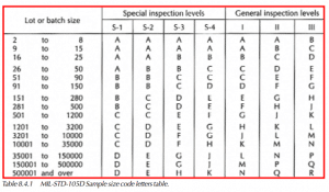
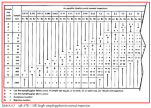
Upon receipt of the incoming material, we must determine the size of the shipment and the specified AQL level to be used, which in our case will be 1.0. In our example, we have received 10,250 pieces. Refer to Table I in MIL-STD-105D (Table 8.4.1). Move down the Lot or batch size column until the lot size range of 10001 to 35000 is found. Move horizontally across the table until reaching the General inspection level II column. Note the letter “M” in our example. Continue on to Table II-A in MIL-STD-105D (Table 8.4.2). In the Sample size code letter column, find the letter M from the previous table. The next column, Sample size, lists how many samples to take from the lot. This is 315 pieces in our example. Remember, these samples must be pulled at random from the lot. We said previously that we would use an AQL of 1.0. Move horizontally across the table to the AQL column labelled 1.0. The value 7 is found in the accept (AC) area and 8 in the reject (RE) area. This means that if 7 or fewer defective samples are found, the lot is acceptable. If 8 or more defective samples are found, then the lot is rejected.

If we find an arrow in the AQL column for our sample size code letter, we must follow the arrow in the direction it is pointing. When the first set of accept/reject values is reached, we must move horizontally back to the sample size column and use that size for our inspection. For example, if we were using sample size code letter D and an AQL of 0.65, we run into an arrow pointing down. Following the arrow, we find we must use a sample size of 20 and accept/reject values of 0 and 1.

Further detailed information on how to use the other sampling tables and switching rules can be found in the MIL-STD105D booklet. Grant and Leavenworth also have a great deal of information in Part 2 of Statistical Quality Control, 5th edition.

Single, Double, and Multiple Sampling

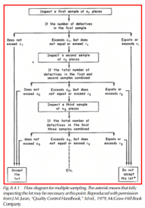
Many sampling plans offer a choice of single, double, or multiple sampling. In single sampling plans, a random sample of n items is drawn from the lot. If the number of defectives is less than or equal to the acceptance number, c, the lot is accepted. If not, it’s rejected. In double sampling plans, a smaller initial sample is drawn, and a decision to accept or reject is made if the number of defectives is either quite large or quite small. A second sample is taken if the first is inconclusive. Since it is only necessary to draw second samples in borderline cases, the average number of pieces inspected per lot is fewer than with single sampling. In multiple sampling, one or more still smaller samples are taken until a decision is finally reached. This process may result in fewer inspections, but is more complex to administer. Figure 8.4.1 diagrams a multiple sample plan (Juran, 1979, p.24-5).

Double or single plans simply stop at Special Inspection Levels A or B in the diagram respectively. In double or multiple sampling plans, the probability of acceptance is more difficult to calculate. It is also more difficult to calculate for a variables-type plan. In the case of the most frequently-used plans, such as MIL-STD-105D, Dodge-Romig, and Bowker and Goodes, OC curves are given selectively for single, double, and multiple plans. Care should be used in drawing conclusions from published OC curves because they may not be plotted on comparable scales. However, in general, it is possible to derive single, double, or multiple sampling schemes with OC curves. (Western Electric, 1956, p.242, Juran, 1979, p.24-1 and 24-24, and Juran/Gryna, 1970, p.418.)

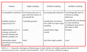
Table 8.4.3 summarizes comparative advantages and disadvantages of single, double, and multiple sampling. In cases where the cost of inspection per part is high, the reduction in number of pieces may justify multiple sampling despite higher administrative costs. On the other hand, single sampling is preferred if minimallytrained operators are used or other costs are high.

Characteristics of Effective Sampling Plans

Good acceptance sampling plans have several characteristics. They are listed below and elaborated in following subsections (Juran/Gryna, 1970, p.418).

• The sample selection must be thoroughly described to assure that parts are randomly chosen. 
• The quality index (AQL, AOQL, etc.) is chosen to reflect real needs of the consumer and producer. In concept, the AQL should not call for a higher quality than actually required. It should represent a balance between the cost of achieving higher quality and the cost of permitting a lower level. In practice, it is a compromise between vendor capability and buyer requirements. 
• The sampling risks are realistically shared between producer and consumer according to quantitative terms. Sampling tables can be used to match required producer’s risk with consumer’s risk. If tables don’t work, special sampling plans can easily be devised. Producer’s risk is defined broadly as the probability or risk of a normal product being rejected by inspection. Consumer’s risk is that of accepting product when the lot quality is relatively poor. (The Statistical Quality Control Handbook, by Western Electric Co. Inc., 1956, discusses these concepts in detail.)
• The total inspection costs are minimized. A complex set of costs can only be approximated because the primary and secondary costs depend on agreed-upon procedures.
• The ancillary knowledge, such as process capability, vendor data, etc., is built into the plan. Sampling data (either past or present) is only one source of information concerning probable acceptability. For example: 

1) Vendor’s test data, operator’s measurements, automatic machine records (these can be validated through the concept of decision audits and used to further understanding) 

2) Scientific and/or engineering knowledge pertinent to the process 

3) Separately acquired data on process or machine capability — for example, the standard deviation

There are no general procedures for defining how such data is used to alter published sampling tables. However, where specific knowledge exists, it may well improve or simplify the plan.

• The plan is sufficiently flexible to reflect pertinent changes. Flexibility is a definite asset. MIL-STD-105D has been noted as an example of a very flexible plan (Juran/Gryna, 1970, p.425).
• The measurements taken are exact and repeatable. Any quality measuring process loses credibility if it is not repeatable. Measuring tools must often be specially designed to ensure ease of use and accuracy of measurement. Automatic recording of data and conversion of data to computer format further reduces the likelihood of error and greatly speeds up the process.
• The measurement data becomes a data base for both short- and long-run process control. Modern computer technology makes it relatively easy to catalog and store process and audit data. If collected data is converted to computer format and transmitted to a larger computer with an appropriate software, archival record storage is not difficult.
• The plan is simple to explain and easy to administer. Some plans have gone some distance to achieve ease of understanding, but at the time of this writing, much remains to be done. Modern computer technology has much to offer in this regard.

Sampling Bias

When sample selection is left to human choice, human biases can inadvertently intrude. Here are some examples:

• Sampling from the same location in all containers 
• Selecting only samples that appear to be defective or acceptable 
• Choosing samples that are easily accessible

There is a classic story of an inspector who always picked samples from the four corners of each tray, and the knowing production operator who carefully placed perfect product in each corner. Structured sampling plans assume randomness. To avoid distortions from biases, sampling must be planned. Once a plan is chosen, it must be policed to ensure that actual sampling occurs according to plan (Juran, 1979, p.24-7, and Juran/Gryna, 1970, p.434).

Sampling Plans Based on Prior Quality Data

Conventional sampling plans assume that the frequency distribution of sampling lots follows classical probabilities of occurrence. In short, they ignore any previous knowledge gained on the past quality sampling. If this knowledge could be rationally applied to future sampling processes, it should reduce sample sizes and, thus, inspection costs. This is called the “Bayesian” approach, after the Bayes Theorem (Juran, 1979, p.24-33). A Bayesian plan generally requires a smaller sample than does a conventional plan with equivalent risk factors. But this is not always true because the assumption that prior distributions can be applied to present sampling practice is not always valid. Oliver and Springer have developed “Bayesian Sampling Plans” that provide sample size and acceptance criteria for single and double sampling plans (AIIE Technical Papers, 1972, p.443). They do so by incorporating data on the quality of previous lots into the sampling tables. The methodology is straightforward:

• Collect quality data on previous lot sizes of N and sample n. Calculate the fraction defective (p) in each sample. 
• Calculate the average fraction defective (p), and the standard deviation of fraction defective using the basic formulas.
• Define the values for AQL, LTPD, and the corresponding producer’s and consumer’s risks. 
• Read the plan from the tables.

Juran and Gryna, in their book, Quality Planning and Analysis, 1970, page 435, illustrate that this technique does indeed result in smaller sample sizes. There is considerable literature available on this subject (see references at the end of this chapter). Hald provides an extensive analysis of sampling plans based on prior product quality distributions (Technometrics, 1980, pp. 275-340). He also questions the assumption of transference of past data to present situations.