What is the True Position Analysis of Geometric Tolerancing

As mentioned earlier manufacturing is caught between two conflicting corporate directions; statistical process control, and geometric dimensioning and tolerancing. Each of these directions taken alone makes logical sense and is desirable. Taken together, they may be very difficult (if not impossible) to achieve.

Geometric tolerancing is a desirable system because: 

• it clearly defines form, orientation, profile, and run out; 
• it clearly defines datum features; and 
• it clearly defines tolerance zones.

True position tolerancing is a sub-part of geometric tolerancing that deals with location. True position tolerancing uses coordinate dimensions to indicate an exact position and defines a circular tolerance zone at that exact position.

Positional characteristics all have at least one thing in common: their location can be described in free space with the descriptors X and Y. In true position analysis, we are concerned with a population of data in the form of (X, Y) coordinate pairs that most likely come from some coordinate measuring machine (CMM), whether comprised of hard (fixed) or soft (touch probe) gauging. 

Ordinarily, true position tolerancing is suited only for functional gauging in that it produces no variables data, as required for x-bar statistical process control charts. Functional gauging does not tell a skilled tradesperson in which direction to adjust the process.

True position analysis seeks to overcome the shortcomings of functional gauging with a graphical tool that allows the operator to view the data two-dimensionally. At the same time, it provides readouts that tell the operator what direction and how far to move the process. Any time the measurement of more than one particular item (e.g., X and Y) must be made to determine the state of a process, there exists the very real probability that the univariate charts for X and Y alone will yield conflicting results.

The approach taken in DataMyte’s true position analysis sub-system is to use bivariate normal probability statistics, which have the effect of integrating the elliptical (X,Y) coordinate pair population with the circular tolerance zone, producing an estimate of the percentage of parts expected within specifications. Once this estimate is in place, Cp, Cr, and CpK values may be calculated.

True Position Analysis: Polar Deviation

In its simplest form, the polar deviation chart is an extension of the scatter chart (with ‘Display Nominals’ = Yes) that is already in DataMyte: SPC software. Beyond the scatter chart, there are two significant extensions to create a polar deviation chart:

• Display the data as a two-dimensional geometric zone (ellipse) 
• Show bonus tolerance if applicable.

As an example, consider the measurement of a bore (or a boss). With inspection observations as to the location of this diametric characteristic yielding coordinate pairs of (X, Y) values, we plot these points on a chartesian coordinate system display. In other words, our result is a square display area broken into four quadrants by the nominals for X and Y, and the inspection samples shown as (*) where the X and Y coordinates meet.

Once this is achieved, we next average all our Xj’s and Yj’s and find the Xa and Ya (average center location). Next, we compute n *Sigma(Xj) and n *Sigma(Yj) to yield our insigma tolerances and plot an n-sigma ellipse around the data values themselves.

Once the data points are plotted on our “bull’s-eye” chart, we next overlay the engineering specification limits for ± nsigma tolerances and plot an n-sigma ellipse around the data values themselves.

When these data points are plotted on our bull’s eye-like chart, we next overlay the engineering specification limits for ± X and ±Y, which are drawn as a circle (X and Y must be bilateral tolerances). If this diametric characteristic is an RFS feature — that is, if the tolerance for this bore or boss is the same Regardless of this Feature’s Size (or radius/diameter) — then we are essentially done.

All that remains is to compute the difference between the nominal (X,Y) and (Xa,Ya) for our transpositional readout, and the angle of the vector formed from nominal (X,Y) to (Xa,Ya) for our rotational readout. These readouts can then be output to a multi-axis machine tool as correction offsets for making the next lot of parts.

Bonus Tolerance 

If, however, our bore (boss) is an MMC characteristic — that is, Maximum (or Minimum) Material Condition feature — the calculation process gets a little more complicated. First, MMC features are those minority of characteristics on a GD&T blueprint that can be a little off-center, as long as they are a little oversized in the case of bores, or undersized in the case of bosses. With this situation, the individual center location (X,Y) is adjusted with the same piece’s radius or diameter deviation from its nominal.

Thus, the net effect is that we get an MMC circle (outside of the RFS circle) plotted on our bull’s-eye graph. The space between these circles is called bonus tolerance.

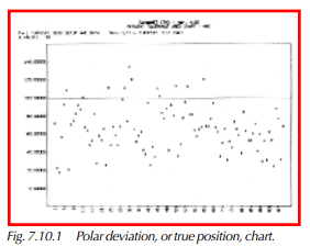
The Polar Deviation chart includes the following numeric readouts for the user 

(see Figure 7.10.1):

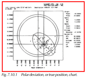
• Origin (Major, Minor), 
• Specs (RFE, MMC), 
• Means (Major, Minor), 
• Ellipse – Rotation, 
• Percent in (RFS, MMC, Ellipse, Plot), 
• Cpk of plotted population. 

The chart’s header contains the part number and the list of X, Y, and R features shown on the plot, as well as the number of samples (s) displayed on the chart.

True Position Analysis: Percent Tolerance Used 

The percent tolerance used (PTU) chart is, in fact, an individuals chart for GD&T characteristics, except that the viewer is interested in the amount of tolerance that each (X,Y) for RFS or (X,Y,R) for MMC consumes. Therefore, the upper limit line on the plot is the 100% line, and each measured bore or boss tolerance used is displayed as an asterisk (*). This graph is most useful when deciding whether using bonus tolerance will buy you anything.

The PTU chart (see Figure 7.10.2) lists the part number and feature names in the header, along with the number of samples plotted. Along the vertical axis of the chart are the percentages (0 to 120 or more) of tolerances used. Along the horizontal axis are the sample numbers (1 to # VALUES) in increments.