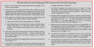
What are gauge Capability Studies

All gauges and test equipment have inherent variability. Whether this measurement error (capability) precludes using a given gauge for a statistical analysis in a specific application can be readily determined using an established methodology.

Consider a sample study: five parts, three inspectors, one gauge, a single control dimension, and two sets of readings. (The following is reproduced with permission from Industrial Quality Control. See the reference at the end of the chapter.)

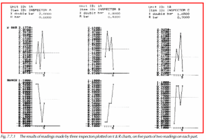
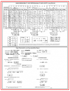
Five parts are selected and a single dimension specified for measurement. The parts are then numbered sequentially, 1 through 5. Three inspectors are selected; each uses the same gauging instrument, and measures the parts in a random order to assure that any drift or change will be spread randomly throughout the study. When the first set of readings is obtained, the inspectors measure a second set in a random order. To eliminate the possibility that one inspector could bias another inspector’s reading, the individual conducting the study should be certain that no information is exchanged. Figure 7.7.1 shows the results plotted on an average and range chart. The readings and results will be carried forward and used as a sample capability study.

gauge Repeatability 

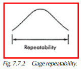
Repeatability is the variation obtained when one person, using the same measuring instrument, measures the same dimension two or more times. See Figure 7.7.2. In this example, only two measurements were made on each piece, or a sample size of 2. The standard deviation for these values can be estimated using the average range. In control chart applications this is done using the formula below:

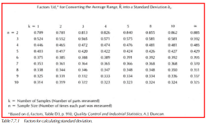
The factor d2 is essentially independent when the number of samples, k, is larger than 10 or 15. For smaller k values, Table 7.7.1 gives corrected 1/d2 factors.

Calculating the estimated standard deviation within parts for each inspector in Figure 7.7.1 (repeatability) gives the following results:

Inspector A
R = 0.6
1/d2 = 0.840
σˆ (within parts) = (0.840)(0.6) = 0. 504
(d2 is taken from Table 7.7.1 — Sample size is 2, and 5 parts were measured.)
Inspector B
R = 0.4
1/d2 = 0.840
σˆ (within parts) = (0.840)(0.4) = 0.336
Inspector C
R = 0.7
1/d2 = 0.840
σˆ (within parts) = (0.840)(0.7) = 0.588

Assessing these results individually, Inspector B has the least variation and the best repeatability. Assuming, however, that all three inspectors normally perform this gauging operation, a standard deviation can be calculated using the average range for all three: 

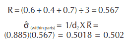
Note that for d2, k has changed from 5 to 15. From Table 7.7.1, 1/d2 = 0.885.

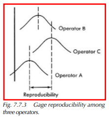
gauge Reproducibility 

Reproducibility is the variation in measurement averages (between inspector variation), where:

See Figure 7.7.3. The 1/d2 factor is based on one sample, with a sample size equal to 3. From Table 7.7.1, this value is 0.524. Then,

Statistically, variances can be combined to give a single value according to the formula:

This resultant value would be used to measure the repeatability and reproducibility, or 

It is immediately apparent that reduced variability could be attained by inspector training, which could minimize the differences in averages, or by obtaining a more precise gauging device.

Assume the total tolerance for the parts used in this study is 3.0. A 99% spread factor is chosen to provide a high confidence level for the gauge repeatability and reproducibility. The tolerance consumed by the measuring system is calculated using this formula:

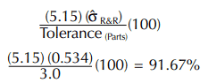
The constant, 5.15, is derived from the Table of “Areas Under the Normal Curve” (Appendix, Table A-3). The constant represents a 99% confidence level that any gauge R&R readings with these parts, equipment, and operators would fall within the same range of variability.

This percentage (91.73) cannot be directly associated with the percent good parts rejected or the percent bad parts accepted. The situation is undesirable, however, since the accepted standard for gauge capability is approximately 10% or less of the total tolerance

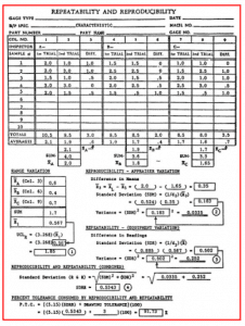
The same information is shown in Figure 7.7.4, using a standardized form that simplifies the calculations required. (This is a form developed by a major automotive manufacturer.) All of the calculations given above are transferred and shown on Figure 7.7.4. Figure 7.7.6 shows the same type of information as Figure 7.7.4, but Figure 7.7.6 shows the long method of calculating. What follows is the sequence of operations needed to complete this standardized form.

Measurement Error Effect on Acceptance Decisions 

Previous mention was made concerning the effect that measurement error had on accepting defective material or rejecting good material. This aspect was explored by Alan R. Eagle. (See the references at the end of the chapter.) The general concept is shown graphically in Figure 7.7.5. In this illustration, the gauge or testing device is zeroed on the upper and lower specifications, and the measurement errors are distributed about these points.

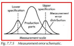
It is obvious that, due to these errors, a probability exists that a good part could be rejected or a bad part accepted. Several assumptions were made in calculating the probabilities involved (a normal practice in statistical analysis):

• The distribution of production parts is normal.
• The parts are centered on the blueprint nominal. 
• The specifications intersect the parts distribution at +2 standard deviations. 
• The measurement error distribution is normal and distributed about the 0 setting.

Using curves developed by Eagle, it is shown that a gauge which consumes 91% of the specified tolerance would only accept 1.45% defective parts on the low end, and would reject about 7% of good parts on the high side. Since these would logically be re-inspected before final rejection, relatively few errors would be made.

In Quality Planning and Analysis (see the references at end of the chapter), a rule of thumb is given:

If the ratio of 3 standard deviations of measurement error to product tolerance is less than about 25%, then the effect of measurement error on decisions can usually be ignored.

For situations where the specifications include more than ± 2 standard deviations of the parts, the graphs overestimate the actual probabilities. For the converse situation, i.e., less than 2 standard deviations are included in the specifications, the graphs underestimate the actual probabilities. This latter condition would indicate that the major problem exists in the machine or process, not the gauging.

xists in the machine or process, not the gauging. If the process is not centered or not normal, errors would also exist and the problem would have to be solved by other methods. Simulation is one technique that could be used if the conditions warranted such an approach. Also, if the gauge is used to obtain data for control chart purposes, the fact that the process mean fluctuates could produce results that would have to be individually analyzed.

This method was presented primarily to reveal that the percent tolerance consumed by repeatability and reproducibility should not be judged solely by its magnitude, but must be further evaluated to determine its effect on potential decision errors.